Excerpt from Chapter 3: The Basics of Estimating Wage or Salary Loss
Economic/Hedonic Damages: The Practice Book for Plaintiff and Defense Attorneys
by Michael L. Brookshire and Stan V. Smith
The Concept
The $856,115 loss estimate in Table 7 is still not the appropriate loss estimate in most circumstances.
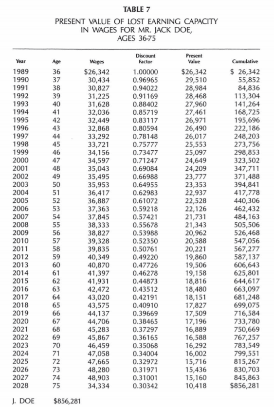
It assumes a 100 percent probability that Mr. Doe would have been alive, participating in the workforce, and employed in each and every year through his life expectancy of age 75. While this is possible, it is not probable.
The estimate of lost earning capacity in wages must be adjusted for work-life expectancy if the measure of economic dames is what we expect that Jack Doe would have earned. Somehow, the loss figures must be lowered to reflect the major probabilities that might have kept Jack from continuous, full-time work over his life.
Before turning to issues relating to how work-life reductions should be made, a more fundamental issue should at least be mentioned.
Wrongful death statutes and appellate court opinions often directly refer to lost earning “capacity.” Forensic economists have assumed this to meant that likely earnings are a stream of earnings through work-life expectancy, rather than through the longer period of life expectancy.
Yet, a dictionary definition of “capacity” is, “the maximum amount that can be contained; the maximum or optimum amount of production…”6
When we speak of plant capacity, we mean the maximum production of a manufacturing plant, without regard to the expected utilization of the plant as a percentage of its maximum production.
Unless statutes or appellate court opinions specifically refer to the need for consideration of work-life expectancy as they discuss lost earning capacity, then the legal parameters within which the forensic economist must work are unclear. It can be argued that the term “earning capacity,” or the term “earning power,” implies that work-life expectancy reductions should not be made.
Indeed, work-life probabilities address the likelihood that full earning capacity will not be achieved by a person at a specified age.
Traditional Approaches
Until recent years, work-life expectancy tables, developed and published by the U.S. Department of Labor, were based upon census data.
These tables might tell us that a Jack Doe, dead at age 33, had a work-life expectancy through age 62.
An economist would then refer to the cumulative column of Table 7 below, look up the total through age 62, and estimate that the expected value of loss for Jack Doe would be $644,617.
Such work-life tables are seriously flawed.
They assumed that once Jack Doe began participating in the workforce, he would continuously do so through age 62. This was a particularly serious error for women, who frequently exit and enter the workforce.
These work-life tables also assumed a 0 percent chance of unemployment.
Finally, they did not differentiate work-life expectancy by such important variables as race and educational level.7 In a 1982 article, the leading U.S. Department of Labor expert on work-life expectancy stated that these tables were obsolete.8
The Bureau of Labor Statistics of the Department of Labor replaced these tables in 1982 with so-called “increment-decrement” tables of work-life expectancy.9 These tables corrected one major problem in the existing tables. They allowed for the fact that persons enter and exit from active participation in the workforce before they finally retire, die, or become permanently disabled.
Work-life expectancy is also broken down by such relevant variables as race, sex, and whether the person was active (participating) or inactive in the workforce at the time of injury or death.
Mr. Jack Doe was a 35-year-old white male, active in the workforce, at the time of death. The most recent increment-decrement tables give Jack another 25.3 years of working life, or through the age of 60.3.
Referring again to Table 7, the expected loss through age 60 is a present value of $606,643. Yet, even these new increment-decrement tables retain significant shortcomings when applied to projections of expected earnings loss. They assume a zero percent chance of unemployment for a typical person over the entire period of his life in which he desires to have a job.
In other words, these tables assume that anytime one wants a job, one will obtain a job and keep it. This assumption is not consistent with reality.
Secondly, these U.S. work-life tables give a number of years—25.3 for Jack Doe—beyond an injury/death date for which earnings should be projected. Actually, chances of less-than-perfect work-life exist at each age and vary importantly by age.
Those who use increment-decrement tables delay the impact of work-life reductions until the end of a working life.
When the net difference of the Teeter-Totter is negative—as has been true for years—this understates the work-life reductions, and overstates economic damages, compared to a technique which assigns work-life reductions to each successive age of the injured or deceased worker.
This problem in the application of U.S. work-life tables can be substantial, especially for female workers.10
The Life-Participation-Employment Technique
The Concept in Illustrative Case
Discontent with the flaws of traditional work-life tables led to the development of the Life-Participation-Employment (LPE) technique for adjusting loss estimates by work-life expectancy.
It was recognized that existing U.S. Department of Commerce and U.S. Department of Labor data—disaggregated by age, race, and sex and updated annually—would allow an economist to adjust loss estimates by the three major variables affecting the duration of working life:
- Probability of Life (L) — Mr. Jack Doe would not have earned the wage figures in Table 7 had he died in any future year. We know from the U.S. Department of Commerce statistics the probability that Jack, as an average white male, would live to and through each future age.
This “L” statistic of life expectancy becomes the first adjustment to the overall LPE technique. - Probability of Labor Force Participation (P) — Even had he lived, Mr. Doe would not have earned the wage figures in Table 7 if he retired, become disabled, or for some other reason not participated in the workforce at any age. We know from the U.S. Department of Labor data the probability that an average white male will participate in the workforce (either has a job or be attempting to find one) at each age.
This “P” statistic is the second adjustment for work-life expectancy. - Probability of Employment (E) — Mr. Doe would not have earned the wage figures in Table 7 if he had been unemployed for any part of any year through his life expectancy. We know from the U.S. Department of Labor the probability that an average white male may be employed at each age. It should also be noted that historical periods of 10 years or more may be averaged for the “P” and “E” statistics so that a “quirky” year in the economy will not bias the expected value estimate.11
One must be alive (L) to participate (P) in the economy, and one must be participating to have a chance of being employed (E).
Therefore, the product of the three distinct probabilities at each age—the joint probability LPE—is the chance that an average person would actually have been alive, trying to find a job, and in fact, employed.
In Table 8, the previous loss estimates for Mr. Jack Doe are lowered by these LPE probabilities at each age. By multiplying the previous present value estimates by these probabilities, we are further reducing the loss estimate by all of the major life risks to which Mr. Doe would have been exposed—the risk of death, of disability, of ill health, of unemployment, and the chance of early retirement.
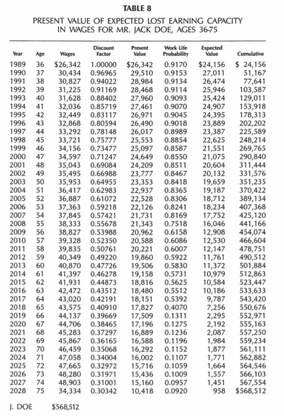
It is clear from Table 8 that these work-life expectancy reductions using the LPE technique are significant.
By his late 50’s, Mr. Doe’s present value numbers are multiplied by approximately 60 percent and therefore lowered by approximately 40 percent. After age 65, the present value estimates are lowered by 85 percent or more.
The expected (present) value of the lump-sum loss is the $568,512 lump sum in Table 8, versus $644,617 or $606,643 alternatives using existing U.S. work-life tables.
The LPE technique may lower loss estimates even more, in percentage terms, depending upon the race and sex of the plaintiff.
On the other hand, an application of the LPE technique can greatly raise the value of loss estimates in partial disability cases.
For More Information…
- Explore more chapters of the textbook.
- Download Chapter 3 [PDF, 7.38 MB].
Read additional sections from Chapter 3 of The Practice Book for Plaintiff and Defense Attorneys:
6 – The American Heritage Dictionary (Boston: Houghton Mifflin Company, 1982), p. 236
7 – See Michael L. Brookshire and William E. Cobb, The life-Participation-Employment Approach to Worklife Expectancy in Personal Injury and Wrongful Death Cases, For the Defense (July 1983), pp. 20-25.
8 – Shirley J. Smith, New Worklife Estimates Reflect Changing Profile of Labor Force, Monthly Labor Review (March 1982), pp. 15-20.
9 – Ibid.
10 – For more background on these issues, see David M. Nelson, The Use of Worklife Tables in Estimates of Lost Earning Capacity, Monthly Labor Review (April 1983), pp. 30-31; George Alter and William Becker, Estimating Lost Future Earnings Using the New Worklife Tables, Monthly Labor Review (February 1985), pp. 39-42; and Shirly Smith, A Comment, Monthly Labor Review (February 1985), p. 42.
11 – AS will be seen in Chapter 7 on Special Cases, historical averages are not used to project participation rates for average females.